Beginners Tutorial
This tutorial provides a basic overview of the image processing workflow of the CowSuite. A test dataset is provided for this tutorial.
The GUI
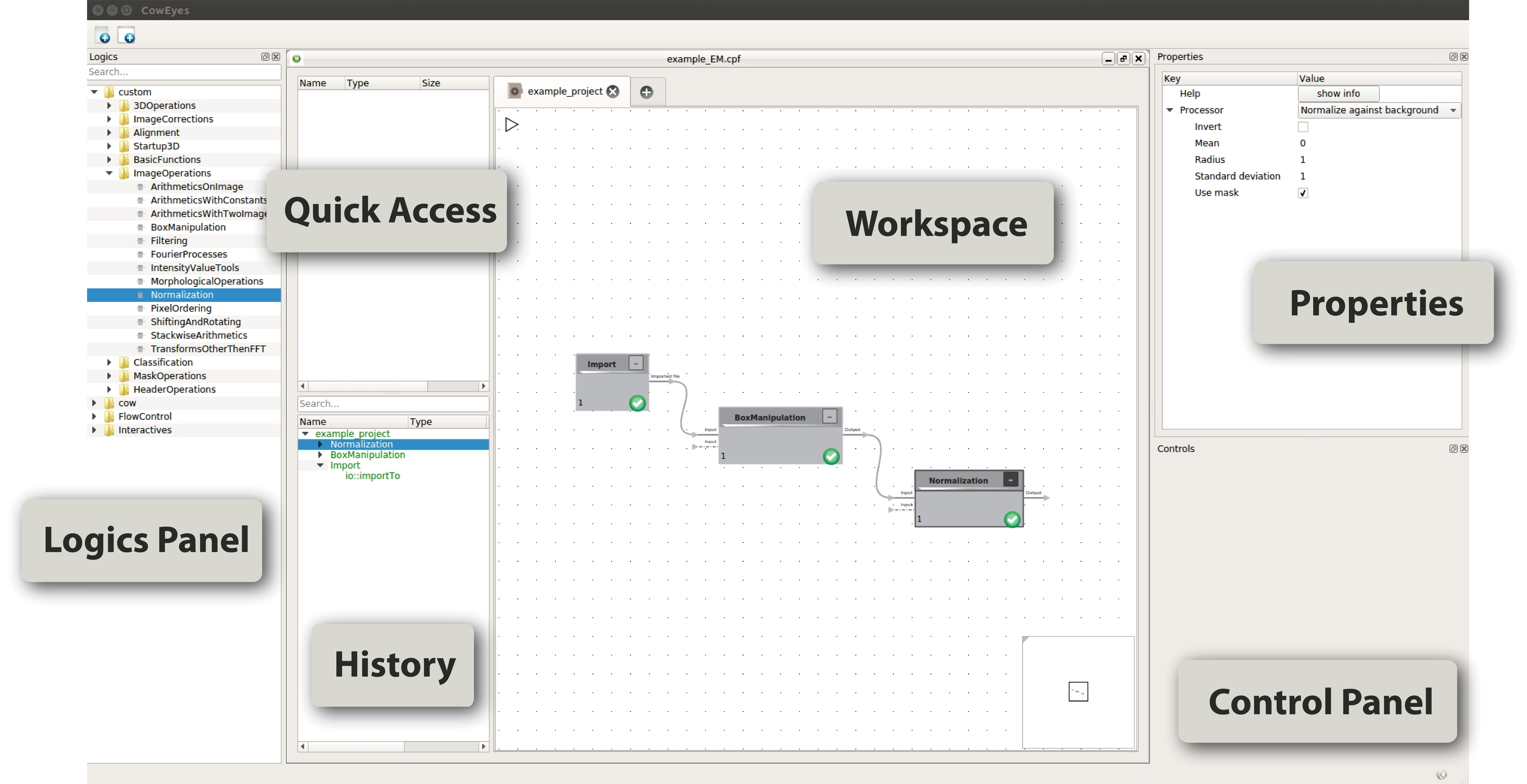
The basic sections of the Cow's graphical user interface (GUI) are the following:
Workspace: To open a new project, click on the + symbol (“New Project”) at the top-left corner of the GUI. Name your project and specify the filepath where you would like to store it. Open a new workspace (this is where the logics will be stored; see Logics Panel) by clicking the + symbol in the top-middle portion of the screen. To zoom, simply click on the white area in the middle of the screen and use the zoom bar that appears in the top-right portion of the screen.
Logics Panel: Specific functions in the Cow are arranged in logics, which are the basic units of the image processing workflow. Logics are arranged in logics groups according to their function on the left-hand side of the GUI. Logics are dragged and dropped into the Workspace for visual programming. The Logics Panel can be easily navigated with the search bar at the top of the Panel. Note: For an in-depth explanation of a particular logic, please see the Logics
Quick Access: When working with multiple tabs in the Cow, you can copy-and-paste logics from the History window and store them in the Quick Access window. Just go to the History box, then click and drag the desired logic into the Container above. If the logic has already been run, then it will retain the information it has processed when stored in the container.
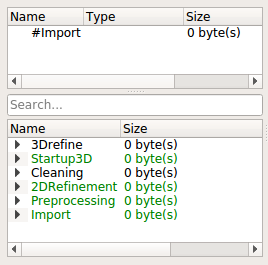
History: To easily keep track of your workflow, every logic you use is logged in the box on the left-hand side of the GUI. This log can be easily navigated using the search bar immediately above it.
Properties: When a logic has been placed in the workspace, it often needs to be adjusted according to your preferences using the Properties window. To access this window, click on the logic in your workspace. The Properties window appears at the top-right corner of the GUI.
Control Panel: The Control Panel appears directly under the Properties Window when you are working with logics that offer interactive viewers (e.g. those used for 3D reconstructions).
Step 1: Import data
To start a project you first need to import your data. The Import logic loads your data into the Cow.
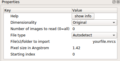
- Import: Find the Logic Group entitled BasicFunctions. Click and drag the Import logic into your workspace. Click on the logic in your workspace and specify the properties of your data with the Properties window. For this tutorial, use the following settings: Dimensionality = Original, Number of images to read = 0, File type = Autodetect, File(s)/folder to import = (specify location of your data), Pixel size in Angstrom = (varies), Starting index = (varies).
- Click the “Play” icon in your workspace to run the program.
Step 2: Preprocessing
During preprocessing your data is prepared for 2D classification.
- Coarsing: Find the logic group ImageOperations. Click and drag the BoxManipulation logic into your workspace. In the Properties window, select “Coarse” and set the Coarse factor to 3. Connect the BoxManipulation logic to the Import logic. Note: if using multiple tabs in the GUI, simply click and drag the desired logic from the History window into the Quick Access window. Click the “Play” icon to run the new logic.
- Filtering: Find the logic group ImageOperations. Click and drag the Filtering logic into your workspace. In the Properties window, apply the following settings:
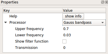 Connect the Filtering logic with BoxManipulation of the previous step and click the “Play” icon to run the new logic.
 - Normalization: Select Normalization from ImageOperations In Properties apply the settings shown below. Connect with Filtering from the previous step and click “Play.” The output of Normalization is your set of preprocessed particles.
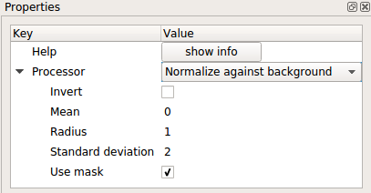
Step 3: 2D operations
Generation of references
- Reference-free classification: Select Principal Component Analysis (PCA) logic from the Classification logic group. In Properties apply the following settings: Dimension = 100, Eigenimages = Disable, Using mask = Disable. Connect Principal Component Analysis (PCA) with Normalization from previous step and click “Play.” Now select the Classification logic and apply the settings shown here. Connect with Principal Component Analysis (PCA) logic from previous step and click “Play.” The output of the Classification logic contains your class averages.
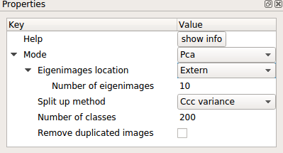
- Extraction of good classes: Find the logics group entitled interactives and select Extract Use the Classification logic of the previous step as the input (this contains your class averages). Then select Contouring (also from the interactives group).
- Optimize references: Under the Alignment logics group, select OptimizeReferences and apply the settings shown here. Connect the “io:out” node of the previous logic with the input of OptimizeReferences logic.
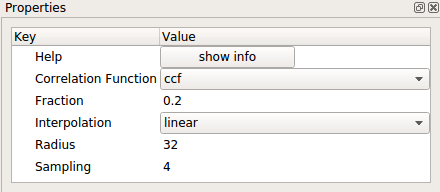
- Mass alignment: From the Alignment logics group select the MassAlignment logic. Set the Pixel threshold = 0, Circular mask fraction = 1. The ouput of MassAlignment contains your references.
Reference-free alignment
- Select the Alignment logic and apply settings shown below. Use your preprocessed particles (the output of Normalization; see Step 2: Preprocessing) as your “input images.”
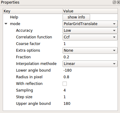
- Select another Alignment logic from the Logics Panel and set to mode = AppendAliInfos. Use the “AliInfos” output of the previous logic as the input for “Align Infos” and use the “Output” of the Normalization logic (see Step 2: Preprocessing) as the input for “Images.” The output of the final Alignment logic is your set of aligned particles. (If this is your first round of classification, skip the next step and move to Iteration.)
Alignment with reference
- Repeat steps 1-4 from Generation of references to generate another set of references. Use the newest references each time but always use the original preprocessed particles.
- Use new references (i.e. the output of each iterative MassAlignment) as the “Align Infos” for the Alignment logic.
Step 4: Dataset cleaning
After evaluation of your dataset using alignments and classifications you may want to exclude particles contributing to less well defined classes in your dataset. To do so, you may first use the interactive Extract logic to select poorly defined class sums, or those showing artefacts like hole borders, ethane blobs, etc. and then the ExtractByMember logic to exclude particles from your dataset that contribute to these bad class sums.
Step 5: 3D startup
- Angular reconstitution: In the Startup3D logics group, select AngularReconstitution. Apply the following settings: Mode = Euler, Sinograms = None, Symmetry = (varies). Use selected class averages as the input for the AngularReconstitution logic. Click the “Play” button to run the logic. The output of the AngularReconstitution contains class averages with angular information.
Step 6: Refinement
This Step is currently under construction.

