Random Conical Tilt (RCT)
The CowSuite offers the option to analyze random conical tilt (RCT) data. The following tutorial provides a step-by-step guide of how to use the Tilt Mode function. Be sure to check out the CowPicker Shortcuts and Hotkeys for easier navigation in the CowPicker.
Tilt Pair Selection
- Open the CowPicker. Load micrographs by clicking on the folder icon in the top-left corner of the GUI. Select “Tilt mode” and then either “Folder” or “Files” (depending on how you've stored your data) when prompted. Following the prompts, first select untilted data and second select tilted data. Make sure that the files are in .tif format before proceeding.
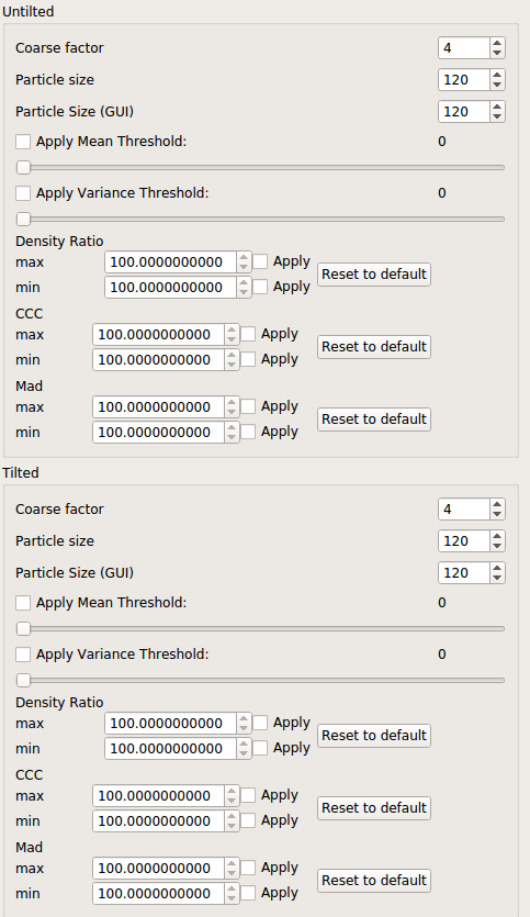
- Open “Settings.” If working with negative stain samples, make sure this box is checked. Click on one of the micrographs to make a test selection, then adjust “particle size” in “Settings” until the circular selection is the same size as your particle. (To delete a selection, right click on it.) Ensure that the settings for “particle size” of the tilted and untilted micrographs are identical, as below:
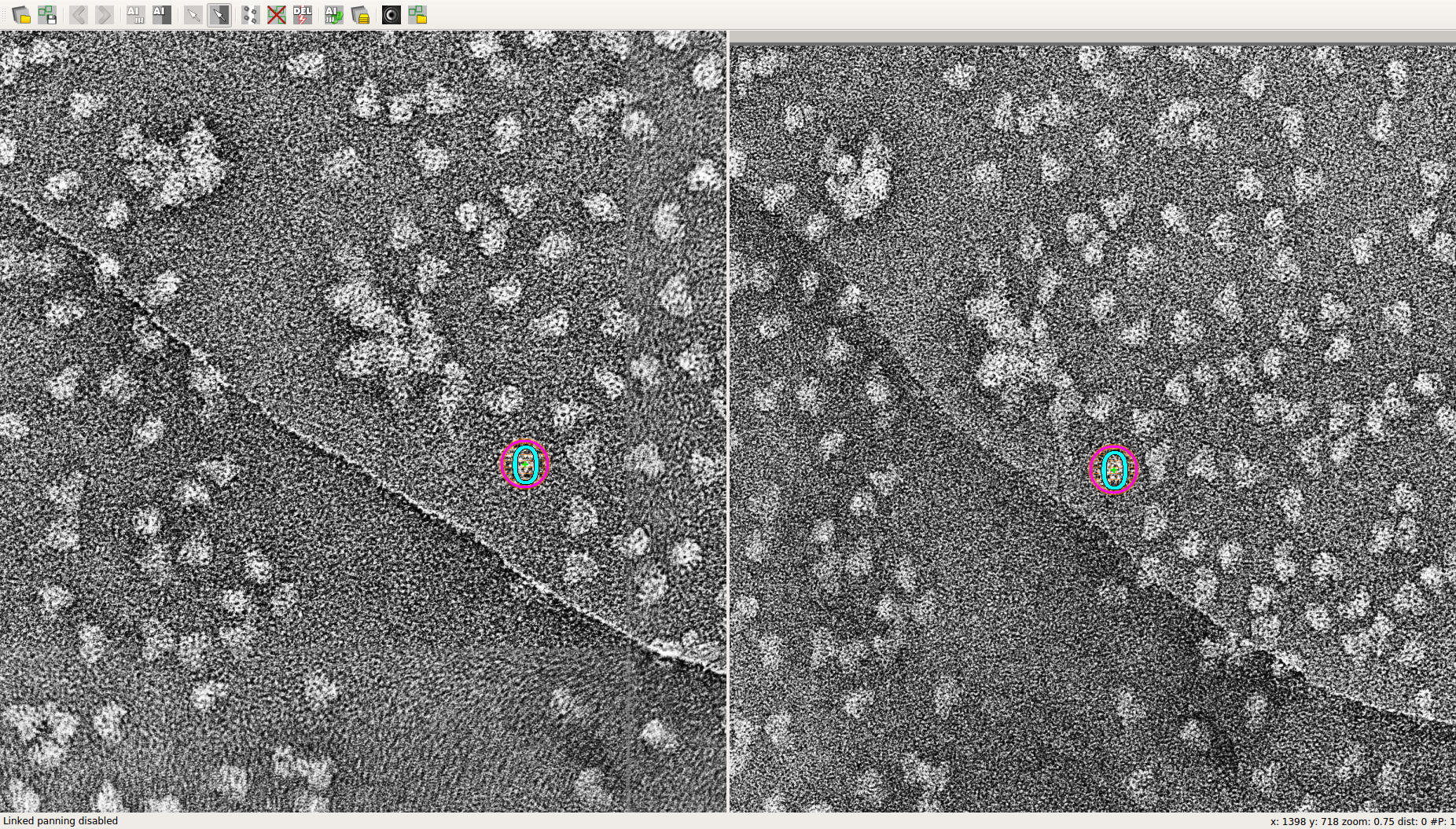
- To make a tilt pair selection, select a particle in one of the micrographs and then find the corresponding particle in the remaining micrograph. Zoom by holding down Ctrl and then moving the mouse wheel. To move the micrographs independently, click on the icon immediately to the left of the red X in the toolbar (shortcut: Ctrl+L).
- Save your progress periodically by clicking on the floppy disk icon in the toolbar. Select whether you would first like to save tilted or untilted data. Select the destination where your data will be stored and create a unique filename for both the tilted and untilted data, since the data will be saved as a separate .plt file for each dataset.
- Once all of your tilted pairs are saved as .plt files, you are ready to preprocess them for import into CowEyes.


Tilt pair cropping
- In the options menu of the CowPicker above the graphical toolbar, go to Extras > Special Crop Operations > Crop from Plt.
- Select the .tif file containing your untilted/tilted micrographs. Select the corresponding .plt coordinate files. Select the destination folder where you want to store the output.
- Decide whether you want to match images and plt files by filename. If the filenames are the same but with different endings, click “Yes.” If the filenames are different, click “No.”
- Enter the cropsize you wish to use. This should match the cropsize used in the “Settings” window that you used in tilt mode.
- Select the filetype that you wish the cropped files to have.
- Click “Yes” when asked “Keep images with plt coordinates which result in black images?”
- Your tilt pairs are now cropped using .plt coordinates and are ready to be imported into CowEyes for further analysis.
Analysis of tilt pairs in CowEyes
- Click on the Import in your workspace and apply the following settings: Dimensionality = Original, Number of images to read = 0 (this setting reads all images), File type = Autodetect, File(s)/folder to import = (select output file containing croppped files from Tilt pair cropping procedure above), Pixel size in Angstrom = (varies), Starting index = 0.
- Run the logics by clicking the “Play” button.
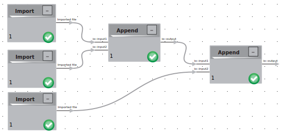
- If working with more than one set of tilted pair files of the same sample, you may want to combine your data. To do so, find the Append logic and drag it into your workspace. Connect this logic with your imported data. Continue this process until all of your data for untilted or tilted particles is combined into a single Append logic (i.e. at the end you should have two Append logics; one for tilted data and one for untilted data). At this point, your logics should be connected as shown by the following:

Tilted Data
- From this point, work with tilted data until otherwise noted. You will deal with the tilted and untilted data separately. Once the data is appended, it needs to be filtered. Find the Filtering logic and connect it with the Append logic. Click on the Filtering logic and apply the following settings: Processor = Gauss bandpass, Upper frequency = 0.6, Lower frequency = 0.04, Show filter function = unchecked, Transmission = 0. Click the “Play” icon to run the logic.
- Next select the Normalization logic and connect it to the Filtering logic of the previous step. Click on the Normalization logic and apply the following settings: Processor = Normalize against background, Invert = (select yes if micrographs were acquired in negative stain).
- Find the Random conical tilt (RCT) (random conical tilt) logic and connect the output of Normalization to “io:tilted” input of the Random conical tilt (RCT) logic. Before running the Random conical tilt (RCT) logic, click on it and adjust the settings as shown below (note: pixel size varies):
 At this point, your logics should be set up in the following way:
  Note that the input labeled “io:untilted” has not been connected. Your untilted data must now be processed.
Untilted Data
- Repeat steps 1-2 from the instructions for Tilted Data.
- Perform 2D operations as listed in the Beginners Tutorial. Once you have a 2D classification, connect the “output” of your Classification to the “io:untilted” input of the Random conical tilt (RCT) logic. Click the “Play” icon to run the logic.