Advanced Tutorial: Energy Landscape determination
In this Tutorial you learn how to make and visualize conformational trajectories based on PCA. The method is also described in Haselbach, Schrader et al.. Apart from basic functionalities of the Cow this tutorial requires the use of flow control elements.
Import of Data
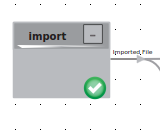
Input for the analysis should be several 3D Volumes, that have the same size and are aligned on each other. To gain these we recomment the use of relion in combination with UCSF Chimera. Once a set of these 3D volumes is created they can be imported into the cow in one go by having them all in the same folder.
Principle Component analysis
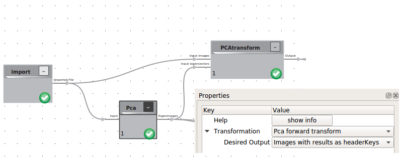
To systematize the conformational flexibility given by the set of 3D Volumes we will use the Principal Component Analysis (PCA) logic. This procedure is heavily depended on the number of eigenvolumes you want to create and the boxsize of your 3D classes. For a standard PC we recomment to calculate less than 20 Eigenvolumes in volumes no bigger than 100 x 100 x 100 voxels. To achieve this the volumes can be downsampled within the cow.
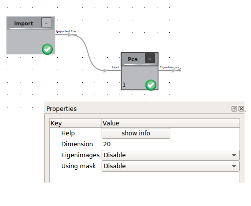 The result of the PCA is a stack of eigenimages, including the average structure and the applied mask as prelast and last item.
Creation of Eigenimage trajectories
To visualize the trajectories we have to calculate the linear factors for each 3D using the PCA transform logic. The calculated linear factors will be written into the header of each image. To now visualize the trajectories we will now use the flow control.
Preparation of the Input Data
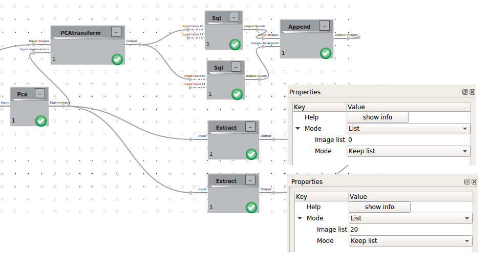
As Input for the flow control we need the average structure and the eigenimage we want to visualize. To gain these we use the extract logic.
Additionally we will need the min and max values of the linear factors with respect to the chosen eigenimage. Those can be extracted using the the SQL logic with the following query:
SELECT * FROM t0 WHERE linearFactorForEigenimage0 =(SELECT MIN(linearFactorForEigenimage0) from t0)
SELECT * FROM t0 WHERE linearFactorForEigenimage0 =(SELECT MAX(linearFactorForEigenimage0) from t0)
For more convenience within the flow control we will append those two value carrying images
Flow control
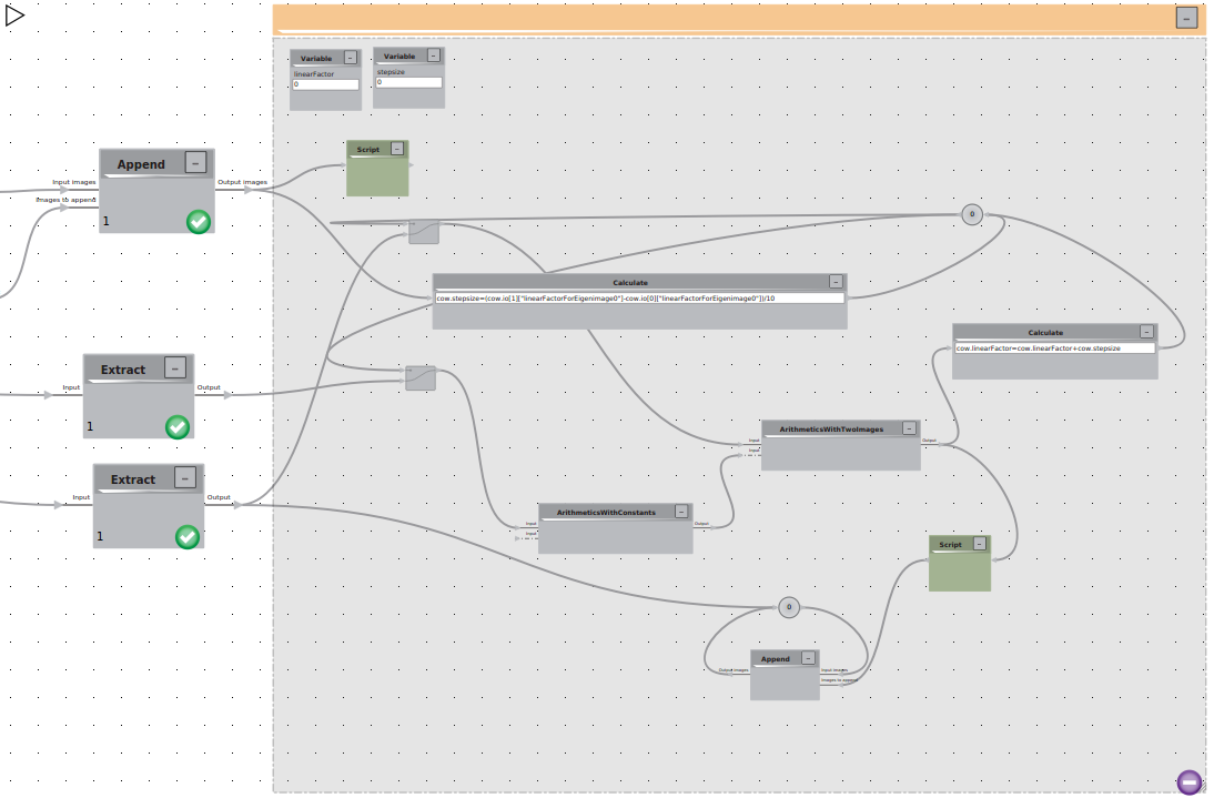
First we need too initialize two variables linearFactor and stepsize.
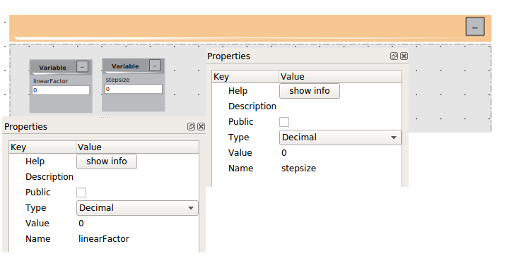
Than we will build two loops:
We will initialize the linearFactor as the minimal Value using a script
cow.linearFactor = cow.io[0][“linearFactorForEigenimage0”]
To visualize 10 intermediate structures we calculate the stepsize with a Calculate tool with
cow.stepsize=(cow.io[1]["linearFactorForEigenimage0"]-cow.io[0]["linearFactorForEigenimage0"])/10
We will use this calculation to trigger our first loop that should run for 10 iterations. The loop itself should trigger the reading of the two inputs: the total average and the eigenvolume of choice using two bypass elements. The eigenvolume is modified by multiplication with the current linearfactor and than added to the average image. After successful calculation the linearfactor is modified with a calculate element.
cow.linearFactor=cow.linearFactor+cow.stepsize
In the second loop we calculate append all intermediates on the average structure to convieniently visualize the movement in the 3D viewer. Using a script we add the current linear Factor in the header of the calculated linear combination
temp = cow.io[0]
temp["linearFactor"] = cow.linearFactor
cow.io[0] = temp
and than simply loop over the append logic. The resulting trajectory can be visualized in the 3D viewer.
